Categories
Final Project Final Project

Final Project


http://humn270finalprojecthaipujunjie.blogs.bucknell.edu/

My research question has two parts. For my own part of the research, I want to discover how Trump’s tweets reveal Trump’s information. Are there any trends in his tweets? Are there any habits or routines of his that can be unveiled through his tweets? For the combined part of the research, Haipu and I are interested in finding more information after combing my data with his data, especially to figure out what he focuses most and what the news focus most and whether there is any relationship between his tweets and the news about him.

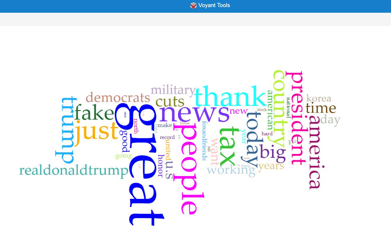
The methodology of my research is basically using python to write code for collecting raw data and extracting metadata. Then, I used Voyant and Palladio to analyze and visualize the data I collected. I used Voyant mainly for text file analysis and used Palladio for metadata analysis.

On the way to the final results, there are a lot of challenges and obstacles. Here are some problems that I encountered and finally resolved on my way.

The first step is to create my corpus. As a good base is crucial to a building, so is a good corpus to a data visualization project. The database I have will play an important role through my progress of the project. Due to my computer science and engineering major background, I decided to use coding methods to collect data from Twitter. Furthermore, since Trump is really popular on Twitter and a lot of people have concerns about him, I decided to use Trump’s tweets as my database. I spent great effort trying to collect the linguistic features and behavioral characteristics of him.

Code for collecting data for the corpus

With the reminder of Professor Faull, I noticed that metadata can also reveal a lot of information and may have unexpected positive effect when combining with raw data. Therefore, I wrote another piece of code for gathering and organizing metadata.

Code for preparing metadata

It’s not the end of the story of data collection. I used this corpus and database for assignment 3 and get some seemingly fantastic visualizations including graphs and timeline.

Palladio Timeline made from data with mistakes

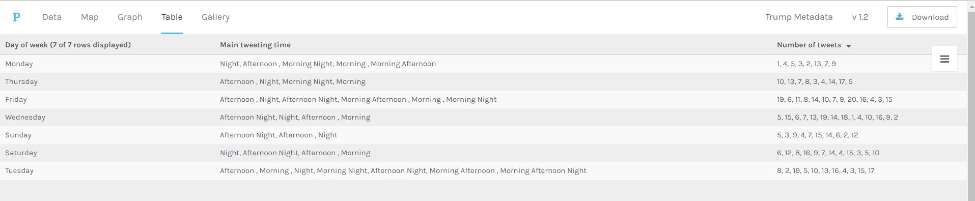
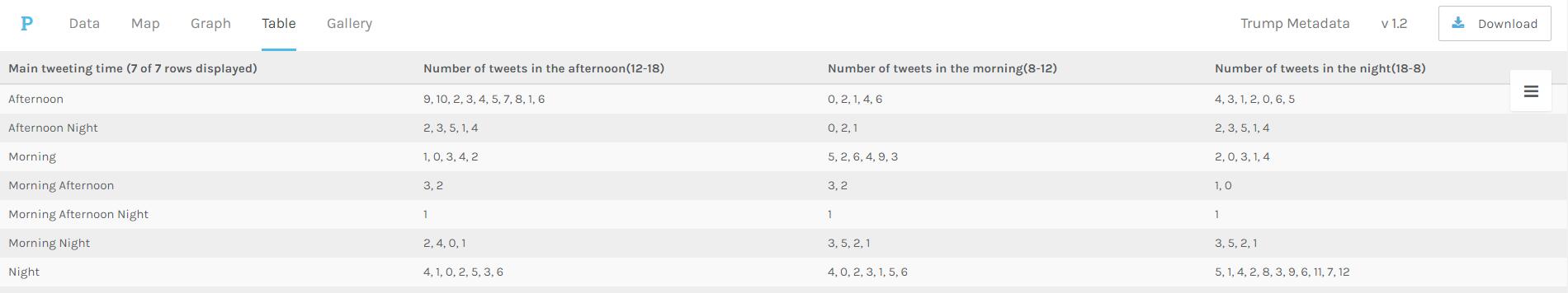
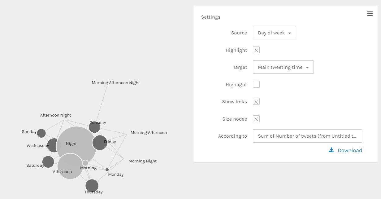
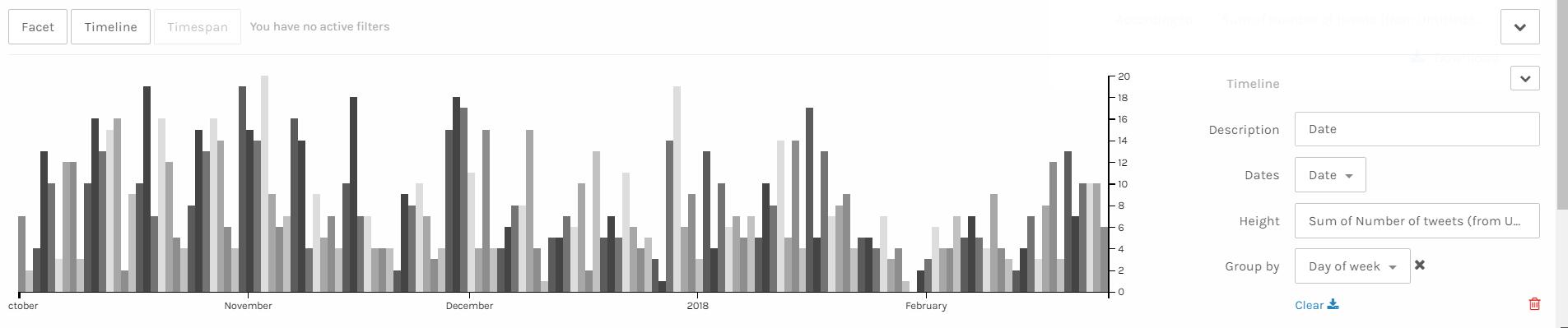
After assignment 3, Professor Faull pointed out that according to some analysis, Trump mostly posts tweets in early mornings. However, my data showed that he post tweets mainly in the night and afternoon, which lead to my attention. After careful analysis, I found that the timezone of the original tweets is UTC, which causes the problem. Therefore, I added the feature of timezone conversion to my code and finally solved the problem. Although the results still show that he post tweets mostly in the night and afternoon, I fixed the original error, thus eventually acquiring the final version of my database. If you compare the above and the below timelines, you can find various small differences. For example, on January 31st, the above timeline shows that there are 2 tweets posted while the below one shows that there is no tweet posted.

Palladio Timeline made from data without mistakes

Through this incident, I learned that it is really important to carefully progress in the process of data visualization. Reading Edward Segel and Jeffrey Heer’s article Narrative Visualization: Telling Stories with Data, I learned that as a storyteller, I am the intermediate between raw data and audience. Therefore, I should take the responsibility for interpreting data as well and correctly as I can.

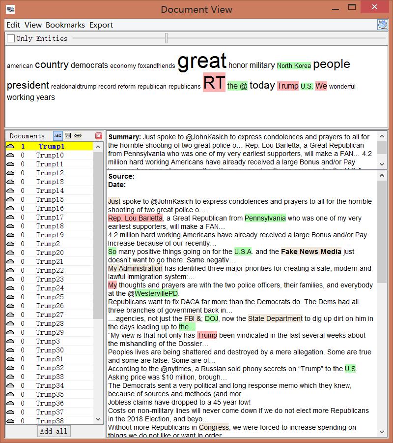
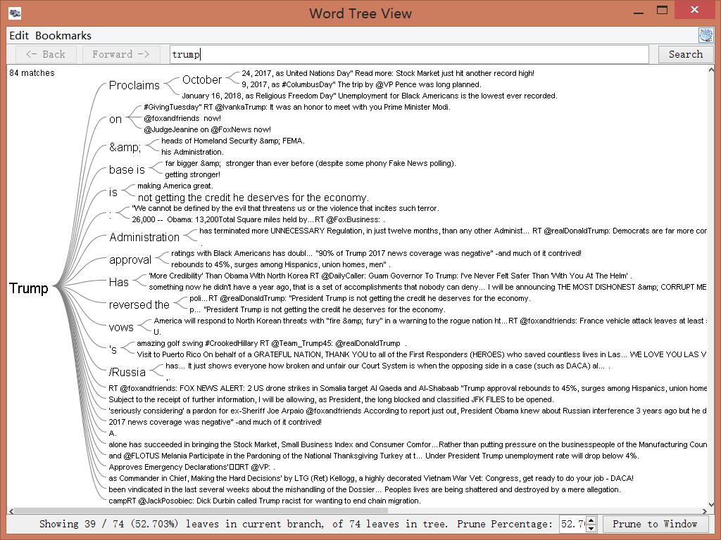
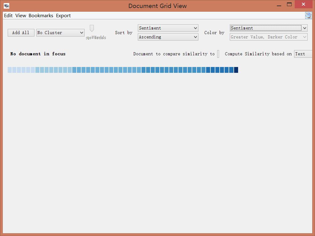
In addition to metadata visualization tools, I also used text analysis visualization tools, like Jigsaw. Jigsaw is helpful when producing word trees and context. The feature I love the most in Jigsaw is the document grid view. This feature provides multidimensional visualization with order and color. Also, since documents are ordered, it makes viewing documents in some organized sequence possible.

Document grid view of Jigsaw

However, there are some pitfalls in Jigsaw. First, the interface of the software is pretty old. Thereby, it’s hard to use Jigsaw to produce good-looking visualizations. Moreover, the functionality of Jigsaw is limited. Compared with Voyant, Jigsaw is unable for the user to choose what they want to see or what they want to ignore. Therefore, I eventually determined to use Voyant and Palladio as my visualization tools.

During the period of analysis, I also faced a problem that I used to use a number to name the files I collected. However, it’s hard for people to understand what these numbers mean and it’s difficult for visualization tools to order them. Therefore, I tried hard to change my code to use the date as an identifier, therefore solving the problem.

Voyant bubbleline visualization without date as identifier

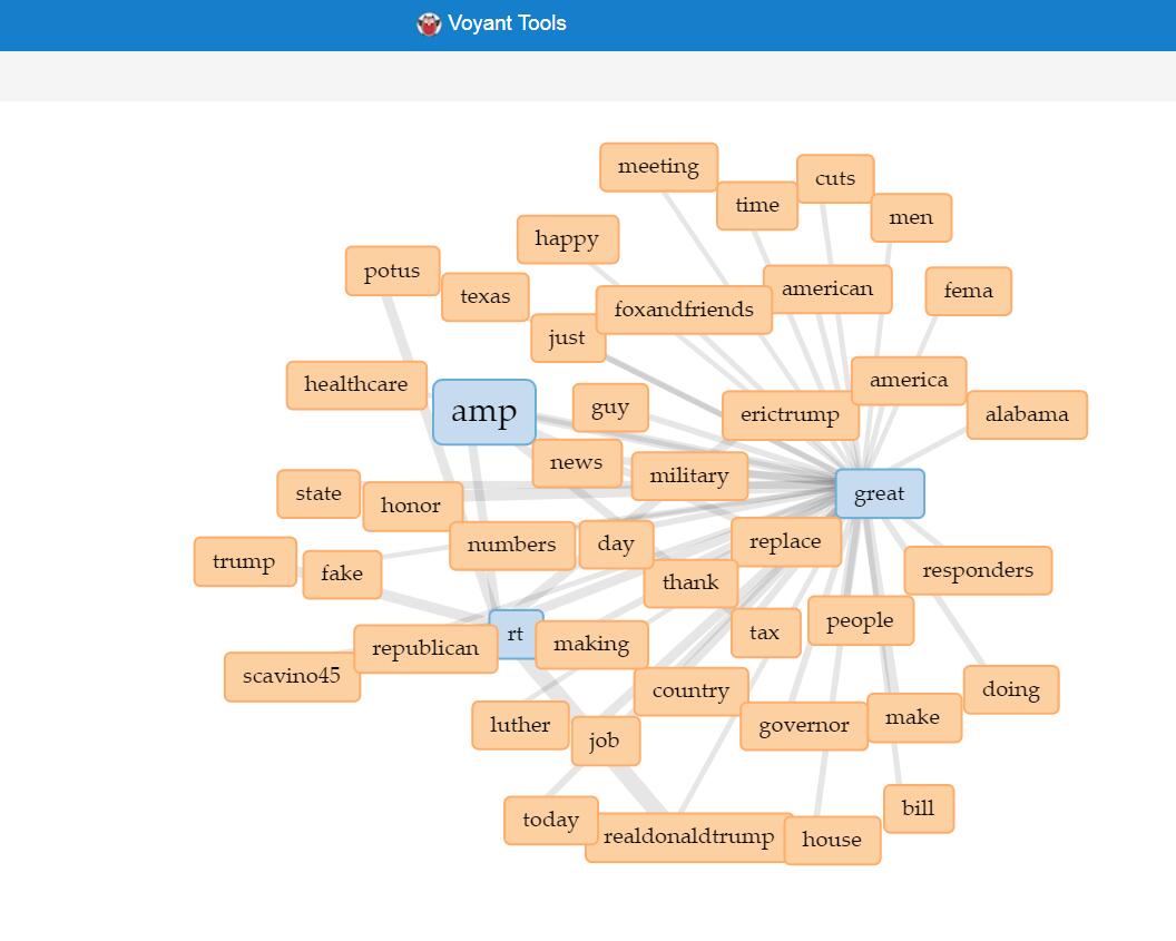
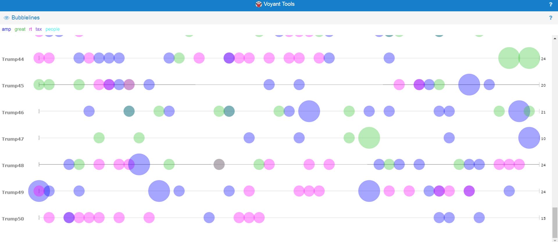
After finishing my part of the research, Haipu and I combined our work together, comparing our visualization produced by Voyant through terms, bubblelines and trends.

We met a lot of problems when combining our work. Since there may be multiple news posted one day but there is only one file for tweets per day, the organization of matching files seems to be really hard. What’s worse, when trying to use excel to combine our data, we found that data on the same line may have different dates, due to different frequencies. In order to circumvent this problem, we decided to construct two timelines separately and then compare the timelines. This solved the problem and provided us with the opportunity to analyze and compare our work effectively and efficiently.

Another problem we met was the software failure of Voyant. When we loaded our data separately to Voyant, we found that the term and trend features did not work properly. Nothing showed up at the context window when I clicked a word and the frequencies shown on the trends were really strange. According to our speculation, it was due to the limit of the number of files that Voyant can handle. Therefore, we were not able to load all of our data to Voyant. Our solution was to divide our data into pieces, specifically into months, and then compare trends of each month. This finally solved our problems.

Despite difficulties and obstacles, we finally reached our goals and fulfilled the project. I found some habits and of Trump and discovered trends in his tweets. Haipu and I together found the relationship between Trump’s tweets and the White House news, illustrating the differences and similarities. To conclude, I feel good with our project because it answers our research questions.

Categories
Assignment 5

Assignment 5

The goal of this assignment is try to understand the data in the Baptized Indians database using Gephi visualizations. I made edges for people with ID 276-325, so all my visualizations have 375 nodes and 75 edges. Below is the default layout of my data sheets when I finished entering the 75 edges to the database.

Default Layout

In this visualization, I can only see some edges between nodes, most of which are thin and two of them are strong. Nearly nothing more can be shown by this graph. From this point, I begin to add features to this visualization.

Color-Modularity

First, I add modularity as a color attribute to this graph. This attribute shows people in different groups, connected with edges I add before. Now, I can see different small communities inside this large group of people in different colors. Moreover,these gray nodes are people that are not connected with others. In other words, they may have relationships with others, but since I only added edges for nodes with ID 276-325, their relationships are not shown in this visualization.

Color-Modularity, Layout-ForceAtlas

In order to view the inner relationship more clearly, I use Force Atlas as the layout. In this visualization, I can easily distinguish different small communities, in which nodes form a connected tree. I can see that the purple group at the top left corner contains most number of nodes, thus learning that Magdalene, represented as the center node in that group, has played an important role in that community.

Color-Ranking-Degree, Layout-ForceAtlas

Furthermore, I use the ranking feature and select degree as the ranking attribute and generate this visualization, in which nodes with deeper colors have higher degree. In this visualization, I can obviously see that the center nodes of the left group and the top left group have greatest influence on the relationship, since their degree are the highest. Also, I can figure out that the middle part of the visualization are the nodes that are not connected.

Color-Nation, Layout-ForceAtlas

Next, I try the nation feature. This attribute seems to be really meaningful, since it is evident that in most communities, people are in the same nations. Therefore, it shows that the native nation is a really important element to the spread of Christianity.

Color-Degree, Size-Betweenness, Layout-ForceAltas

Since I’m not satisfied with two-dimension visualization, I add size as a new dimension. In the above visualization, I visualize degree with color ranking and betweenness with size. The result is really attracting. I can see that nodes with more degree have more betweenness and there are a high-degree class and a low-degree class in most communities. Therefore, I can learn that during the spread of Christianity, active individuals are significant, since they can lead to wider spread. And I can speculate that if more edges are added, the spread will become hierarchical, with some most significant people with highest degree and highest betweenness.

Color-Degree, Size-Eigenvector, Layout-ForceAltas

In the above graph, I replace betweenness with eigenvector value. There are only a few differences between this visualization and the former one. First, I notice that nodes in the left group become larger. Second, nodes in the top right corner become larger. I think it is because eigenvector value takes into account the degree of their adjacent nodes, while betweenness only depends on the degree of nodes themselves. Therefore, the result I can get from this visualization is the same as the above one.

Color-Nation, Size-Betweenness, Layout-ForceAltas

Finally, since betweenness can show degree in some way, I replace degree with nation as the attribute visualized by color. This graph itself can now show a lot of information. First, I learned that nation is an important attribute of the spread of Christianity. In same nations, the spread may be easier. However,  in some situation, spread across nations can happen. It is because that the edges here represent some kind of family relations and it is more probable for people in the same nation to get married with each other. Therefore, I can claim that family relations is also a key element in the spread of Christianity. Second, I observe that the purple nation have the most people who are involved in this database, green and blue coming next. Therefore, I can speculate that Christianity is more popular in these nations than in black or orange nations. Third, this visualization shows that the purple nation tends to have more tightly connected communities, since some groups have large betweenness compared with others. Furthermore, I can identify that the largest node, which is the center node of the group in the top left corner, is the most influential people in this visualization, since this node has the greatest betweenness.


I’m surprised that simple actions on Gephi can reveal so much information in the database. And the beautiful graphs are really fascinating. As described by Edward Segel and Jeffrey Heer, “Crafting successful ‘data stories’ requires a diverse set of skills.” I think using Gephi is such a good skill to learn.

Categories
practice

Visualization Comparison

Categories
Assignment 3

Assignment 3

In the previous visualizations, I simply used 50 files of Trump’s tweets with 30 tweets in each file. This construction of corpus does not provide special meta data and thus is useless when analyzed by Palladio or Google Fusion Tables. In order to make the network visualization make more sense, I reconstructed my data set. My data set is now constructed with Trump’s tweets from 10/01/2017 to 02/25/2018, each file including all tweets posted that day. Also, I wrote code for extracting metadata from the original data set. The main parts of the metadata that I collected are date, day of week, number of tweets, time block in which Trump tweeted most in a particular day and so on. Enlightened by Professor Faull, I think although it’s not feasible to find out the relationship between tweets and events related to Trump, because I did not combine my data with Haipu, it may be interesting to figure out the living habits of Trump if I look into his usage of Twitter during different time blocks and number of tweets in different days of week.

Palladio Table for days of week, main tweeting time and number of tweets

The above visualization shows the relationship among days of week, main tweeting time blocks and number of tweets in a day. It’s obvious that Trump mainly tweets in the afternoon and night on Sundays, which means he might sleep more on Sunday mornings. Also, on Wednesday, Friday and Saturday, he usually tweets more than on Monday and Sunday.

Palladio Table for main tweeting time blocks and number of tweets in different time blocks

The above visualization shows the relationship between main tweeting time blocks and number of tweets in different time blocks. It’s evident that Trump is accustomed more to tweet in the afternoon and night, since there is no number more than 10 appearing in the “Number of tweets in the morning” column. Also, if he tends to tweet in the morning one day, he will not tweet much that day.

Palladio Graph for days of week and main tweeting time grouped by sum of number of tweets

The above visualization can better show the relationship than the table ones. The size and color dimensions definitely provides me with more information. Since the size of nodes ‘Night’, ‘Afternoon’ and ‘morning’ are really different, I can say that Trump tweets much more in the evening than in the afternoon than in the morning. Similarly, I can see that Trump tweets more on Friday, Wednesday, Thursday and Saturday than other days of week.

Palladio Timeline with height as number of tweets grouped by days of week

I think the above visualization is the best among all visualizations I made through Palladio. Since I have my corpus constructed in the order of date, I can easily make a nice looking timeline and see the trend of a period of nearly 5 months. It’s obvious that the number of tweets Trump made has a period. The number of tweets reaches the climax in the middle of week and declines after that and rises again when a new week begins. Also, it’s obvious that he tweets more in last year than in this year. Especially at the end of January and beginning of February, he tweeted much less than usual, which is strange. Some events might take place during that period and I hope after I combine my data with Haipu’s I can figure it out.

I think these visualizations are actually representations of information. A lot of information may be veiled at the first glance of data. However, after clever organization and visualization, these informative knowledge can be revealed. As discussed above, in the network visualization, the sizes and colors are dimensions that carry critical information. And I can make a guess that the distance between nodes shows how close relationship they have.

Categories
Assignment 2

Assignment 2

For the construction of my corpus, since I am doing a research related to twitter feeds, I’m familiar with tweet collecting procedure and I fully understand that there is much information that can be extracted from twitter feeds. Therefore, I determined that my corpus should focus on President Trump’s public twitter feeds. I downloaded his tweets through Twitter API and I have 50 files in total, each file containing 30 tweets. With this corpus, I can anticipate interesting findings like Trump’s main focus in the past months. Also, with my computing experience, I successfully scrapped off some useless and meaningless content from the original corpus such as urls.

Since these two platforms possess a number of functionalities, I chose some of the most important ones and made snapshots. Also, in order to compare these two platforms, I selected some similar and some different visualization tools.

Document in Jigsaw
Word Graph in Voyant

These two visualizations are created using two similar tools, which produce views of frequently used word in documents with different advantages and disadvantages. Obviously, the visualization produced by Voyant is much more beautiful, with the difference of frequencies shown more evidently. However, Jigsaw is superior to Voyant in the way that it shows these words with their contexts, which may provide more information to users.

Wordtree in Jigsaw
Link in Voyant

Since the wordtree functionality in Voyant only provides “America Great Again”, so I used link instead of word tree for Voyant. This functionality, like wordtree, provides information about words and their local relationship. The wordtree visualization in Jigsaw obviously shows the words’ local relationship in context, with different sizes representing different frequencies, which can offer direct knowledge to users. On the other hand, the link feature in Voyant produces better interactive visualization. Once selected the icons in the graph, users can either expand or remove icons, thus enjoying the benefit of iterative visualization. Also, the nice layout and colorful labels make the feature more user friendly.

Sentiment in Jigsaw

This feature is something unique in Jigsaw, not included in Voyant. This visualization shows the sentiment according to text analysis in different documents. Each block represents a file and darker color indicates greater sentiment value, in other words sadness or anger. This grid view tool can also do other analysis depending on different needs. It can produce special insight because it takes two variables into account. For example, it can produce a timeline showing the sentiment by choosing document date and sentiment for “sort by” and “color by” relatively.

Bubbleline in Voyant

This feature is only provided by Voyant, indicating the frequencies of different words in different documents. It can provide direct impression and is convenient for users to compare different files. The lines indicate the text order and different sizes represent the frequencies. Additionally, different colors indicate different entities. Therefore, this visualization includes at least three different dimensions, which provides a thorough and broad view of the data set.


During the process of corpus construction and visualization analysis, I found Tanya Clement’s observation is verified. The first part of her argument is easy to understand. Using visualization platforms, I successfully combined different kinds of information and created some multidimensional viewpoints. For the second part of her argument, I understand that due to the unknown algorithms behind these visualization platforms, the results presented may be biased. Therefore, I should keep in mind that the results may not be exactly correct when I do research using these visualization platforms.

Categories
Assignment 1

Assignment 1

First Visualization
First Visualization

I choose this visualization because it does a fantastic job in dynamic interaction and it looks fancy. “Interactive visualizations, on the other hand, aim to explore available information, often as part of a process that is both sequential and iterative.”(Sinclair, paragraph 2) It is obvious that this visualization provides multiple ways of interaction that can not be fulfilled by static visualization, allowing users to access different information from various perspectives both sequentially and iteratively. Moreover, this visualization uses creative and emergent methods to illustrate the relationship and information in the network. Choosing a center, users can see a relationship network centered with the chosen artist. Clicking on the artist labels, users can further select different options, such as “expand”, “remove” and “create map”. “Expand” and “remove” can increase or reduce the complexity of the network. “Create map” can create a new network centered with the chosen artist. There are different words in the background, which are different attributes that belong to some of the artists in the network. Hovering on these attributes, the artists that have these attributes will be shown, thus providing users with direct and obvious information. Similarly, hovering on artists will lighten the artists’ attributes. To conclude, this visualization provides not only information from different perspectives but also strong interaction.


In order to show some differences between dynamic and static visualizations, I choose this static semantic network visualization as the second one. Although the resolution of the picture is low, it’s easy to see that this visualization uses different dimensions to illustrate information, such as colors of lines, solid or hollow dots and colors of bars. Also, since the visualization is based on a book called “Brave New World”, on the left there is a dimension of different chapters. “For chronological data, the timeline is a venerable visual format, whether manifested statically or interactively.”(Sinclair, paragraph 2) This timeline like feature make this visualization more organized. It is really different from dynamic visualization that static visualization is hard to interact with users. However, clearness and easiness can also make a static visualization helpful and informative.


Third Visualization

For the visualizations in DH Sample Book, I love this visualization most due to it’s easy but nice looking. It is a dynamic visualization that provides various perspectives and fantastic interaction. At first glance, the complex lines may seem to be misleading. However, when hovering on different people, clear relationship will be shown. Furthermore, after clicking them, more text information can be viewed. “That is, some steps come before others, but the researcher may revisit previous steps at a later stage and make different choices, informed by the outcomes produced in the interim.”(Sinclair, paragraph 2) It is evident that users can revisit former steps and make different choices in order to make comparisons and access more information. These interactive, organized and creative ways of understanding the material are really attracting.


Categories
practice

Two visualization selected